The Point of No Return: A Definitive Guide to the Law of Diminishing Returns in Economics and Business

Introduction: Beyond “More is Better”

Imagine a business owner who has just tasted success. The first few employees hired have dramatically increased production. The initial marketing campaign has brought in a flood of new customers. The logical, almost intuitive, next step seems clear: double the inputs to double the success. Hire more staff, pour more money into advertising, and watch the profits soar. This linear assumption—that more is always better—is one of the most common and costly fallacies in business and economics.¹

In reality, every system of production, from a simple farm to a complex software company, operates under a fundamental constraint. At a certain point, adding more resources no longer yields proportional benefits. In fact, it can become counterproductive. This universal principle is known as the Law of Diminishing Returns.

Formally defined, the Law of Diminishing Returns (also called the Law of Diminishing Marginal Productivity) is an economic principle stating that if one factor of production is increased while all other factors are held constant, a point will eventually be reached where the additional output generated from each new unit of input will decline.⁴ It is a law not of failure, but of efficiency, revealing the optimal balance of resources in any productive process.

This definitive guide will explore this crucial concept in exhaustive detail. The journey will begin by building a solid theoretical foundation, defining the essential components of production. From there, the abstract theory will be translated into tangible numbers and graphs, making the law’s mechanics clear and intuitive. The analysis will then move into the real world, examining fascinating, data-driven case studies from farms grappling with fertilizer limits to digital marketers navigating the saturation of online audiences. Finally, these powerful lessons will be distilled into actionable strategies for business leaders, managers, and investors.

The Law of Diminishing Returns is not merely a theoretical constraint to be lamented; it is a powerful strategic tool. Understanding and anticipating its effects is the key to optimizing resource allocation, maximizing profitability, and achieving sustainable, intelligent growth.

Part I: The Theoretical Framework of Production

The Anatomy of Production: Fixed vs. Variable Inputs

To grasp the Law of Diminishing Returns, one must first understand the context in which it operates: the short run. In economics, the “short run” is not a specific length of time, like a week or a year. It is a period during which at least one factor of production is fixed.⁷ This distinction between fixed and variable inputs is the bedrock of the entire concept.

Fixed Inputs are the factors of production that a firm cannot easily alter in the short term. They represent the established capacity of the operation. Examples include the physical size of a factory, the acreage of a farm, a signed lease on a retail space, or essential, heavy machinery.⁸ These inputs define the production environment’s constraints.
Variable Inputs are the factors that can be adjusted quickly to change the level of output. Common examples include the number of labor hours, raw materials, electricity, or advertising spend.⁷ The law examines what happens when we continuously add more of these variable inputs to a fixed set of inputs.

The very presence of a fixed input is not merely a condition for the law but its direct cause. The Law of Diminishing Returns is an inevitable consequence of applying increasing variable inputs to a constrained, fixed resource. This fixed factor acts as a bottleneck. For instance, in a factory with a fixed number of machines, the first few workers can use the equipment efficiently, perhaps even specializing in certain tasks to boost productivity.¹² However, as more workers are added, they must share the same limited machinery. They might have to wait their turn, or the workspace may become so crowded that they begin to get in each other’s way.⁵ The constraint of the fixed factory size is the direct cause of the decline in each additional worker’s productivity. The law, therefore, is not just an abstract observation; it is a description of the physical and logistical realities of a constrained system.

Measuring Output: The Three Pillars of Production Analysis

To observe the law in action, economists and business managers use three key metrics to measure output: Total Product, Average Product, and Marginal Product.

Total Product (TP): This is the most straightforward metric. It represents the total quantity of output—such as tons of wheat, number of cars, or lines of code—produced with a given amount of inputs over a specific period.¹⁵ It is the cumulative result of the production process.
Average Product (AP): This metric measures the overall efficiency of the variable input. It is the total product divided by the number of units of the variable input used. For example, if 10 workers produce 100 widgets, the average product of labor is 10 widgets per worker. The formula is:

AP = TP / L

where L represents the units of the variable input (e.g., labor).¹⁵
Marginal Product (MP): This is the most critical indicator for identifying the onset of diminishing returns. Marginal Product is the additional output generated by adding one more unit of a variable input, while all other inputs are held constant.⁵ For instance, if hiring a fourth worker increases total output from 45 units to 55 units, the marginal product of that fourth worker is 10 units. The formula is:

MP = ΔTP /ΔL

where ΔTP is the change in total product and ΔL is the change in the variable input.¹⁶ The law is often called the Law of Diminishing Marginal Returns precisely because this metric is where the phenomenon first becomes visible.²

The Three Stages of Production: A Visual Journey

As a firm adds more of a variable input to its fixed inputs, its production process typically moves through three distinct stages, defined by the behavior of the marginal product.

Stage 1: Increasing Marginal Returns
In this initial phase, each additional unit of the variable input adds more to the total output than the previous unit. The marginal product is rising.¹³ This occurs because the initial units of the variable input allow for greater specialization and more efficient use of the fixed inputs. For example, in a large, empty kitchen, a single chef is a jack-of-all-trades, running between stations and performing every task inefficiently. The addition of a second chef allows for a division of labor—one preps while the other cooks—dramatically increasing their combined (and marginal) output.¹²
Stage 2: Diminishing Marginal Returns
This is the heart of the law. In this stage, total product continues to increase, but it does so at a progressively slower rate. Each additional unit of the variable input contributes less to total output than the one before it. The marginal product is positive but falling.¹³The fixed input has now become a significant constraint. The business is still getting more output from each new input, but the efficiency gains are shrinking. This is the stage where most rational firms operate.
Stage 3: Negative Marginal Returns
If a firm continues to add the variable input, it will eventually reach a point where doing so is counterproductive. In this stage, adding another unit of input causes total output to fall. The marginal product becomes negative.¹³ This is a state of severe inefficiency caused by extreme overcrowding or oversaturation. Too many workers in the kitchen are now actively obstructing one another, or too much fertilizer applied to a field has become toxic to the crops.² No rational firm would ever choose to operate in Stage 3, as it means paying for more inputs to get less output.

Part II: The Mathematics and Geometry of Diminishing Returns

Calculating the Curves: From Total Product to Marginal Gains

Abstract definitions become clear when applied to a concrete example. Consider a small fast-food restaurant with a fixed kitchen size and a set number of grills and fryers (fixed inputs). The owner wants to determine the optimal number of employees (variable input) to hire for the lunch rush. The output is measured in hamburgers produced per hour.

The following production schedule demonstrates how to calculate Total Product (TP), Marginal Product (MP), and Average Product (AP) as more workers are added, and it clearly identifies the three stages of production.

Table 1: A Fast-Food Restaurant’s Production Schedule

Units of Labor (L)	Total Product (TP) (Hamburgers/hr)	Marginal Product (MP) ($ \Delta TP / \Delta L $)	Average Product (AP) ($ TP / L $)	Stage of Production
0	0	–	–	–
1	10	10	10.0	Increasing Returns
2	25	15	12.5	Increasing Returns
3	45	20	15.0	Increasing Returns
4	60	15	15.0	Diminishing Returns
5	70	10	14.0	Diminishing Returns
6	75	5	12.5	Diminishing Returns
7	75	0	10.7	Diminishing Returns
8	72	-3	9.0	Negative Returns

Source: Adapted from data in.¹²

Walkthrough of Calculations:

Worker 2: Total Product jumps from 10 to 25. The Marginal Product of the second worker is 25−10=15. The Average Product is 25/2=12.5.
Worker 4: Total Product increases from 45 to 60. The Marginal Product of the fourth worker is 60−45=15. The Average Product is 60/4=15.0. Notice that after the third worker (who had an MP of 20), the marginal product has started to decline. This is the entry into Stage 2: Diminishing Marginal Returns.
Worker 7: Total Product remains at 75. The Marginal Product of the seventh worker is 75−75=0. This worker added nothing to total output.
Worker 8: Total Product falls from 75 to 72. The Marginal Product of the eighth worker is 72−75=−3. This worker’s presence was actively detrimental to production, marking the beginning of Stage 3: Negative Returns.

The Geometry of Productivity: Graphing the Law

The numerical relationships in Table 1 can be visualized through a set of classic production curves. This graphical representation provides a powerful, intuitive understanding of the law. The graph is typically shown in two panels: the top panel for the Total Product curve and the bottom for the Marginal and Average Product curves.

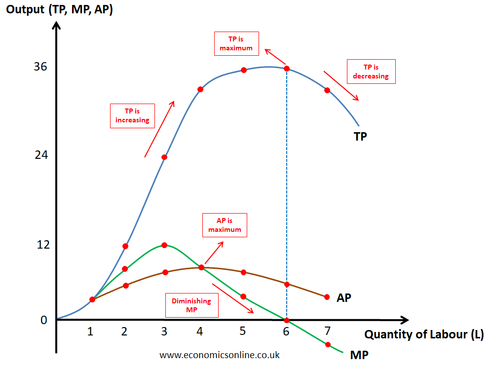
Image Source: https://www.economicsonline.co.uk/content/images/2023/07/Diminishing-Returns-2.webp

Key Geometric Relationships:

The Shape of the Total Product (TP) Curve: The TP curve’s shape is a direct reflection of the Marginal Product.

In Stage 1 (Increasing MP), the TP curve gets progressively steeper.
It hits an inflection point where the MP curve peaks—this is the exact moment diminishing returns begin.
In Stage 2 (Positive but Decreasing MP), the TP curve continues to rise but becomes flatter.
The TP curve reaches its absolute maximum point exactly when the MP is zero.²¹
In Stage 3 (Negative MP), the TP curve slopes downward.

The Relationship Between Marginal (MP) and Average (AP) Product: The MP and AP curves have a precise mathematical relationship.

When the MP is above the AP, it is pulling the average up, so the AP curve is rising.
When the MP is below the AP, it is dragging the average down, so the AP curve is falling.
Therefore, the MP curve must intersect the AP curve at the AP curve’s highest point.²¹

This intersection is more than a geometric curiosity; it serves as a powerful managerial diagnostic tool. The relationship is a universal mathematical rule, applicable to everything from production figures to student test scores. If a student’s average grade is an 85, and they score a 95 (the marginal score) on their next exam, their average will rise. If they score a 70, their average will fall. Similarly, for a manager, as long as a newly hired worker (the marginal unit) is more productive than the current team average, that new hire will increase the team’s average efficiency. The moment a new hire’s marginal product is less than the team’s average, they begin to reduce the overall average efficiency. The point of maximum average productivity—the peak of the AP curve—is precisely where the marginal productivity of the newest hire equals the existing average. This tells a manager the point of peak average efficiency for their workforce. Hiring beyond this point may still be profitable, but the manager must know they are doing so at the cost of declining average efficiency.

A Glimpse into the Calculus (Expert Corner)

For those with a mathematical background, the relationship between these curves can be described with greater precision using calculus. The production function can be expressed as Q=f(L,K), where output (Q) is a function of variable inputs like labor (L) and fixed inputs like capital (K).²⁴

The Marginal Product (MP) is the first derivative of the Total Product (TP) function with respect to the variable input (L).

MP = d(TP) / dL
The point where diminishing returns begins—the peak of the MP curve—is the inflection point of the TP curve. This is where the second derivative of the TP function becomes zero and then turns negative.

d²(TP) / dL² = 0

This mathematical foundation confirms the geometric relationships observed in the graphs and provides a rigorous basis for production analysis.

Part III: Diminishing Returns in the Real World: Data-Driven Case Studies

The Law of Diminishing Returns is not confined to textbooks. It is a persistent force that shapes outcomes in every industry, from the most traditional to the most technologically advanced. Examining data-driven case studies makes the theory tangible and reveals its profound strategic implications.

The Classic Case: Agriculture

Agriculture provides the most intuitive and historically significant examples of diminishing returns, as noted by early economists like Jacques Turgot, Thomas Malthus, and David Ricardo.⁹

Sub-Case 1: The Fertilizer Dilemma

A farmer has a fixed plot of land (the fixed input) and wants to increase crop yield by applying fertilizer (the variable input). Initially, the fertilizer provides essential nutrients that are lacking in the soil, causing yields to increase dramatically. However, at a certain point, the soil and crops can no longer absorb the nutrients as effectively. Each additional bag of fertilizer adds less to the total yield than the previous one. Eventually, excessive application can increase soil salinity or create nutrient imbalances, becoming toxic and actually reducing the harvest—a clear case of negative returns.²

This process reveals a critical strategic insight for any business: the goal is not to maximize output, but to maximize profit. A detailed analysis of wheat production demonstrates this distinction.

Table 2: Optimizing Fertilizer Use for Wheat

Urea (kg/ha)	Marginal Cost ($/ha)	Yield (t/ha)	Marginal Return ($/unit)	Marginal Profit ($/unit)	Total Profit ($/ha)	Analysis
125	$15	3.50	$60.00	$45.00	$530.00	Profitable
150	$15	3.60	$20.00	$5.00	$535.00	Maximum Profit
175	$15	3.65	$10.00	-$5.00	$530.00	Unprofitable Addition
200	$15	3.70	$10.00	-$5.00	$525.00	Maximum Yield

Source: Data adapted from Hudson Facilitation, GRDC.²⁶ Assumes Urea cost of $600/t and wheat price of $200/t.

The data in Table 2 is illuminating. A farmer focused solely on maximizing yield would apply 200 kg/ha of urea to achieve the highest possible output of 3.7 tons per hectare. However, a marginal analysis shows this is a mistake. The additional 25 kg/ha of urea applied to go from 175 kg/ha to 200 kg/ha costs $15 but only generates $10 in additional revenue, resulting in a marginal loss of $5. The point of maximum profitability ($535/ha) is reached at an application rate of 150 kg/ha, which produces a slightly lower yield of 3.6 t/ha. This powerful example shows that rational decision-making requires continuing an activity only as long as the marginal benefit exceeds the marginal cost.

Sub-Case 2: The Crowded Pasture

The law also applies to livestock management. A dairy farmer with a barn of a fixed size (fixed input) might try to increase milk production by adding more cows (variable input).²⁷

Initial Gains: Filling an underutilized barn increases total milk output and cash flow.
Diminishing Returns: As the barn becomes crowded, systemic stresses appear. The average milk production per cow begins to drop, perhaps from 80 lbs to 78 or 77 lbs. While total output is still rising, the marginal return from each additional cow is clearly diminishing.²⁷ This is due to factors like reduced worker efficiency in crowded conditions and increased stress on the animals.
Negative Returns: Severe overcrowding leads to widespread metabolic issues and disease outbreaks (ketosis, displaced abomasums). At this point, the cost of veterinary bills and lost production from sick animals outweighs the milk from the extra cow, leading to a net financial loss. The farmer has entered a “not fun or profitable place to be”.²⁷ This case highlights that diminishing returns can manifest not just as lower output, but also as a decline in quality, health, and overall system stability.

The Modern Factory: Manufacturing and Labor

The quintessential factory example perfectly illustrates the law’s mechanics. Returning to the fast-food restaurant from Part II, the fixed inputs are the kitchen space and equipment, while labor is the variable input.¹²

Increasing Returns (1-3 workers): The first few hires allow for specialization. One worker can manage the grill, another can assemble the burgers, and a third can handle the fryer. This division of labor leads to a rising marginal product as they work together more efficiently than they would alone.¹²
Diminishing Returns (4-7 workers): The kitchen becomes congested. Workers start “bumping into each other”.⁵ They may have to wait for a grill to free up or navigate a crowded workspace. The marginal product of each new worker falls because the fixed capital (kitchen space) is now a bottleneck, even though total hamburger output is still rising.
Negative Returns (8+ workers): The space is now so chaotic that coordination breaks down completely. Workers are actively obstructing one another, leading to mistakes, slowdowns, and a drop in total output.⁵

The Digital Frontier: Marketing and Advertising

In the modern digital economy, the Law of Diminishing Returns is just as relevant, though the inputs look different. For a digital marketing campaign, the variable input is typically the advertising budget. The “fixed input,” however, is not a physical space but a more abstract concept: the size of the high-intent, addressable audience on a given platform.²⁸

Once a campaign has reached the most relevant potential customers (the “low-hanging fruit”), each additional dollar spent must be used to reach less interested or more expensive audiences. This expansion into a lower-quality audience pool is the digital equivalent of overcrowding a factory. The “fixed asset” of the prime audience has been fully utilized, causing the return on investment (ROI) for each marginal dollar to fall.²⁹ Furthermore, repeatedly showing the same ad to a saturated audience leads to “ad fatigue,” where viewers tune out the message, causing effectiveness to plummet.²⁸

Successful companies understand this and develop strategies to counteract it.

Case Study: UNTUCKit’s Audience Expansion

Problem: The clothing brand UNTUCKit experienced rising costs per click (CPC) and costs per acquisition (CPA) on Facebook and Instagram. Their core audience was saturated, and simply increasing their ad spend was yielding diminishing returns.³¹
Solution: Instead of just pushing more money into the same strategy, they changed a different production factor. They used look-alike audience modeling to identify and target new pools of high-intent customers who shared characteristics with their existing best customers. This effectively expanded their “fixed input” of the addressable audience.
Result: This strategic pivot led to a 300% increase in new customer return on ad spend (ROAS), demonstrating a brilliant method for overcoming diminishing returns.³¹

Case Study: FanDuel’s Creative Diversification

Problem: The sports betting company FanDuel noticed diminishing returns on its YouTube ad campaigns, likely due to ad fatigue among its target audience.³¹
Solution: Their approach was twofold. First, they conducted a marginal analysis and discovered that spending 40% of their budget was the most efficient level. Second, to spend more effectively beyond that point, they introduced a diverse range of new ad creatives. This is analogous to a factory upgrading its machinery; they altered another production variable (the ad creative) to increase the productivity of their primary variable input (the ad budget).
Result: The refreshed creative strategy improved results and allowed them to increase their overall YouTube spend profitably, effectively resetting their diminishing returns curve.³¹

Part IV: The Strategic Importance of Diminishing Returns

The Law of Diminishing Returns is far more than an economic curiosity; it is a foundational principle for strategic decision-making in business and finance. Its implications touch everything from day-to-day operational management to long-term corporate strategy and investment analysis.

The CEO’s Compass: Guiding Business Decisions

For business leaders and managers, the law provides a crucial framework for navigating the complexities of growth and efficiency.

Optimal Resource Allocation: At its core, the law is a guide to resource allocation. It forces managers to move beyond asking “What is working?” to the more critical question, “Where will the next dollar of investment or the next employee have the greatest marginal impact?”.⁶ It provides the logic for balancing investments between labor, capital, technology, and marketing to achieve the most productive combination.
Profit Maximization, Not Output Maximization: As the fertilizer case study vividly demonstrated, the ultimate goal of a commercial enterprise is to maximize profit, not simply to maximize production.² The law teaches that the optimal point of production is where the marginal revenue generated by the last unit of input equals the marginal cost of that input. Pushing production beyond this point, even if it leads to higher total output, will erode profitability. This distinction separates strategically sound businesses from merely busy ones.
Informing Cost Structure and Pricing: The law has a direct and inverse relationship with costs. As the marginal product of an input falls, the marginal cost of producing an additional unit of output rises. Understanding the point at which diminishing returns set in is therefore essential for analyzing a firm’s cost structure and making informed pricing decisions to protect profit margins.³³
Sustainable Scaling: The law definitively proves that a growth strategy based on simply scaling up a single input is doomed to fail. Sustainable expansion requires a balanced increase in all relevant factors of production. A restaurant cannot just keep hiring more cooks indefinitely; it must eventually invest in a larger kitchen, more ovens, and more tables. This transition—from adding variable inputs in the short run to expanding fixed inputs in the long run—is the critical distinction between experiencing diminishing returns and achieving returns to scale.¹

The Investor’s Lens: Evaluating Companies

For investors, the Law of Diminishing Returns is a powerful lens through which to evaluate a company’s health, scalability, and long-term potential.

Assessing Scalability: A key question for any investor is whether a company’s business model can scale efficiently. A business that can grow its revenue without its costs growing proportionally is highly attractive. Conversely, a company whose model is constrained by a significant fixed input that cannot be easily expanded is likely to hit a wall of diminishing returns quickly, limiting its growth potential.²⁵
Analyzing Profit Margins: One of the most telling warning signs for an investor is a company that is growing its top-line revenue but experiencing shrinking profit margins. This often indicates that the company is deep into Stage 2 of diminishing returns. It is having to spend more and more (on marketing, labor, etc.) to acquire each new dollar of revenue, a clear sign of operational inefficiency and a potential red flag for future profitability.²⁵

The most sophisticated companies and investors recognize that the ultimate strategy is not just to manage the existing production curve efficiently, but to find ways to jump to an entirely new, more productive curve. An investor should therefore place immense value on a company’s ability to innovate and diversify, as these are the primary countermeasures to the inevitability of diminishing returns in any single core market.

Amazon serves as the quintessential case study in this regard.²⁵ The company’s leaders recognized the eventual diminishing returns in their initial market of selling books online. Instead of merely optimizing their bookstore, they made a strategic leap to a new production curve: general e-commerce. As that massive market began to mature and face its own diminishing returns, they executed another, even more brilliant leap to an entirely different and highly profitable curve: cloud computing with Amazon Web Services (AWS). For a long-term investor, a company’s R&D pipeline and a proven history of successful diversification—its ability to find new “Stage 1s”—is often a more powerful indicator of future value than its current operational efficiency in a mature market.

Beyond Business: Broader Economic Implications

The influence of the Law of Diminishing Returns extends to the highest levels of economic theory and policy.

Historical Context: The law was central to the theories of classical economists. Thomas Malthus famously argued that because the amount of land is fixed, population (which grows geometrically) would inevitably outstrip food production (which grows arithmetically due to diminishing returns on land), leading to widespread famine.⁵
The Counterforce of Technology: What Malthus did not fully anticipate was the power of technology. A significant technological advance—like the invention of the Haber-Bosch process for creating synthetic nitrogen fertilizer ³⁴, or the development of automated manufacturing—can shift the entire production curve upward. This allows for more output to be produced at every level of input, effectively pushing the point of diminishing returns much further into the future.⁴ Technology is the primary force that has, to date, held Malthus’s dire predictions at bay.
Production Possibilities Frontier (PPF): The law also explains the characteristic shape of a country’s PPF—the curve showing the maximum possible production combinations of two goods. The PPF is typically bowed outwards (concave to the origin) because of diminishing returns. As an economy shifts resources from producing Good A to Good B, it first reallocates the resources best suited for Good B. To produce even more of Good B, it must start using resources that are less efficient at that task, meaning it must give up increasingly larger amounts of Good A for each additional unit of Good B. This reflects a diminishing marginal rate of transformation.¹⁸

Conclusion: The Wisdom of Knowing When to Stop

The fundamental lesson of the Law of Diminishing Returns is that in any system, effectiveness is a function of optimization, not maximization. True success is not found in the blind pursuit of “more,” but in the intelligent search for the “sweet spot”—the point where the marginal benefit of an action just equals its marginal cost.¹ Pushing beyond this point is not a sign of ambition but of inefficiency.

This principle transcends economics to become a versatile mental model for decision-making in nearly every domain. It applies to a student deciding how many more hours to study for an exam when fatigue is setting in; to a software engineer determining when further code refactoring yields negligible improvements ³⁵; to a government weighing the marginal benefit of additional regulations against their rising economic cost.³⁶ It is a universal reminder that resources are finite and must be allocated with precision and foresight.

Business leaders and investors are therefore urged to critically examine their own strategies through this powerful economic lens. Where in your operations are you pushing past the point of optimal investment? In which areas have you saturated your “fixed input,” whether it be factory space, market share, or audience attention? And most importantly, where could reallocating that next marginal resource yield a far greater return? The wisdom to know when to push forward and, crucially, when to stop, pivot, or diversify is what separates fleeting success from enduring value.

To continue exploring how production efficiency changes with scale, read our comprehensive guide on Economies and Diseconomies of Scale at uncletj.com.

References and Further Reading

Academic Sources

Brue, Stanley L. 1993. “Retrospectives: The Law of Diminishing Returns.” Journal of Economic Perspectives 7 (3): 185–192. ³⁷
Mold, James W., Robert M. Hamm, and Laine H. McCarthy. 2010. “The law of diminishing returns in clinical medicine: how much risk reduction is enough?” Journal of the American Board of Family Medicine 23 (3): 371-5. ³⁸

Uncle TJ's Blog